Tips for a Smooth R(Studio) Workflow and Reproducible R Code

A lot of people at SESYNC use R (often through RStudio on rstudio.sesync.org), are interested in making their research as reproducible as possible, and want to save time and make life easier for themselves. That’s why I wrote this blog post with some ideas for how you can make your R workflow smoother, easier for you and anyone you ask to help you, and more in line with reproducible science best practices!

Wait, what’s a workflow?

Your workflow, as defined in this tidyverse blog post, is all of your personal habits and preferences that you do as part of any project you work on. It doesn’t include raw data and the code itself. Your workflow is unique to you and you don’t need others to reproduce it, and your project is the actual output you want people to be able to reproduce. Incidentally the blog post I just linked to has some other good ideas for best practices and is worth a read.

Now that we’re on the same page, here are some good ideas for your workflow for R and RStudio. Some tips are SESYNC-specific and some are generally applicable to any time you use R or RStudio.

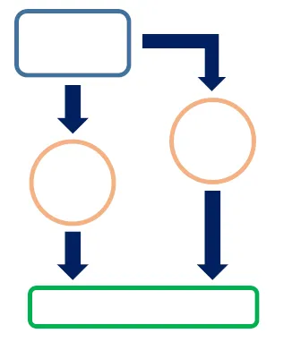
For each topic, I’ve included a “broke” (not recommended practice), “woke” (not bad), and “bespoke” (best practice!) way to do it.

Saving your work

 

Broke: saving your entire workspace

The best practice is not to save your R workspace when you exit R or RStudio. “But wait,” you protest, “what about all the work I did running all that code?” Well, this does not mean you have to unnecessarily re-run any code. If there are specific R objects you want to save from session to session, you should save those objects or export their contents to a CSV. Saving the entire workspace is problematic for a few reasons:

• If anyone else ever helps you with your R code, it will be easier for them to reproduce only the relevant objects rather than an entire “ecosystem” of variables in your workspace.
• It uses up a lot of memory unnecessarily.
• You might have other packages and objects that are interacting with your desired output in ways you might not immediately be aware of.
• It is not explicitly written into a script so it is much harder to reproduce.

It’s easy to set the global RStudio options to not save your workspace by default. Just go to the Tools menu in RStudio and select Global Options and go to the General tab. Set the Workspace options to not restore your .RData automatically on startup, and not to save it on exit, as in the highlighted area in the image below. You can do this both on your local machine and on the RStudio server.

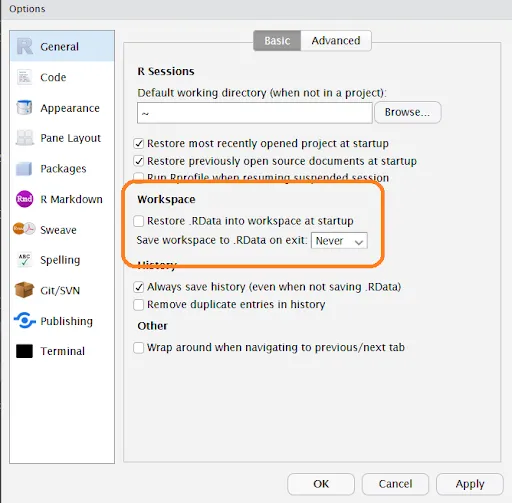
RStudio global options to not save and restore workspaces

If you are running your R script from the command line, type Rscript --no-save --no-restore my_script.R will also tell R not to save or restore any workspaces when your script runs.

Woke: saving individual R objects

Even if it’s a bad idea to save your entire workspace, it’s good to be able to save your progress. This is especially true if you ran a very computationally intensive process that you don’t want to repeat. It isn’t always easy to export things to a CSV. Instead of saving the whole workspace, it is better to identify the object(s) you want to save and save them individually.

You can save individual R objects easily by using the save() function and specifying the names of the objects and the file to write to (usually with the extension .RData). For example,

save(big_object1, big_object2, file = 'my_awesome_output.RData')

In a future session, you can reload the objects by using the load() function:

load('my_awesome_output.RData')

Edit May 2021: I got a comment from a reader saying that an alternative and possibly superior way of saving R objects is to use saveRDS() instead of save(). The key difference is that saveRDS() does not save the name of the object along with it. This can be better if somehow the object name changed in your code between saving and loading, or (worse) you created another object with the same name. Loading your .RData file would overwrite that object. You can save an R object as an .rds file like this:

big_object_reloaded <- readRDS('my_object.rds')

So the upside of saveRDS() and readRDS() is that it avoids potential name conflicts but the downside is that you can only save one object at a time with it.

Bespoke: using RStudio projects in conjunction with saving objects

RStudio includes a feature called “projects” as a way to keep your work in R organized. It is best explained by Hadley Wickham in the project chapter of his book R for Data Science. The basic idea is to keep all the scripts and history associated with one of your real-life projects in one place as an R project. You can switch between them easily. Typically people associate each project with its own version control (i.e., git) repository. I won’t go into too much detail on how to set up projects in RStudio — read the RStudio documentation and the book chapter!

Accessing files in different directories

 

Broke: changing the working directory

A very commonly used function is setwd(). For example many people would set the working directory to their data directory, then read a CSV file from there.

setwd('Z:/data')
data <- read.csv('my_awesome_data.csv')

Unfortunately this is not a great practice because it changes the R environment. This is problematic because it can affect and possibly break other scripts. This is bad enough if you are the only person who will run the script, but if anyone else wants to run your code or help you debug it, it will affect their system as well. They probably don’t have the same directory structure as you do anyway, so the read.csv will return an error. (And don’t even get me started on scripts that start with rm(list = ls()), if you really want to ruin someone’s day.)

Woke: using explicit file paths

A better way is to create a character string with the file path where the data are located. Then you can use the file.path() function to combine the directory name with the file name when you are reading or writing a file.

data_dir <- 'Z:/data'
data <- read.csv(file.path(data_dir, 'my_awesome_data.csv'))

It requires a slightly longer line of code to read a file but is well worth it in saved headaches. If you set the path to the data directory at the very top of the script, it will be easy for others to change it to the correct path on their system.

Bespoke: setting a symlink in your project repository

You can use something called a symlink to allow your scripts to run on both your local machine and the RStudio server without any modification. A symlink is a shortcut to a different directory location that “looks like” a subfolder inside your project’s repository folder. Use the function file.symlink() to create one in R.
For example, if you create this symlink on your git repository for your project on the RStudio server,

file.symlink(from = '/nfs/cooltrees-data/', to = 'data')

and this symlink on your local machine where you have the data directory mapped to the Z drive,

file.symlink(from = 'Z:/data', to = 'data')

you can run your R script in both places without any modification! Remember to add the symlink to your .gitignore so that it can be different on your local and remote copies of the repository.
 

Writing clear and legible code

 

Broke: using opaque variable names and no comments

If you use variable names that aren’t clear and informative, and don’t comment the code, “future you” or anyone else reading your script will have a tough time.

n <- sum(data$status == 0)

No one would know what this code is doing, because the variable names n and data have no meaning, and there are no comments. You probably won’t even remember a few weeks from now!

Woke: using good variable names and commenting your code

Use consistently formatted and informative variable names. Some prefer snake_case and others camelCase for formatting variable names — this thread shows that there are a lot of differing opinions. It’s up to you, but consistency is important to minimize typos and errors caused by entering the wrong variable name. It’s crucial to annotate your code with comments, too.

n_dead_trees <- sum(tree_data$status == 0) # Count the number of dead trees

Now the code is pretty much self-explanatory, but we also include a comment to make things doubly clear.

Bespoke: using RMarkdown to create a document with text, images, and code

RStudio is not only good for writing plain R scripts. You can also create RMarkdown documents which let you combine R code, output, images, and text into a nicely formatted document! This is great for two things: you can richly annotate your analysis, making it easier for you to revisit it later, or you can communicate your results to others. Check out our lesson on RMarkdown to get started, if you haven’t used RMarkdown before.