Date
tl;dr: This post walks you through making a map of the 50 United States with ggplot2, where Alaska and Hawaii are moved from their true geographic locations.
For a recent project, I wanted to make a choropleth map of the fifty United States with Alaska and Hawaii displayed as insets (not in their true geographic locations). It’s a little bit cumbersome to make inset maps in ggplot2 and usually requires a few different package dependencies.
Image
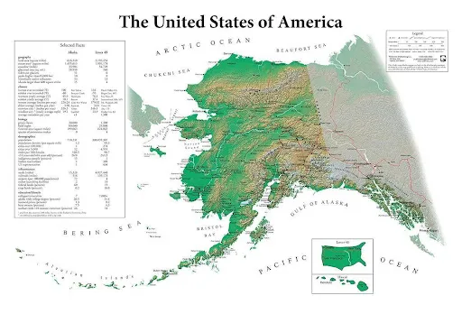
Alaska gets revenge for always getting shrunk down and stuck in the corner.
An alternative that doesn’t require any inset maps is to do a custom transformation on the polygons representing Alaska and Hawaii to magically move them somewhere off the southern “coast” of Arizona. The excellent R package urbnmapr already includes R objects of class sf that have USA state and county boundaries transformed in this way. That allows you to make maps with the geom_sf() function from ggplot2.
But what if you don’t want to use state or county boundaries? For example you might want to plot a map with ecoregion or watershed boundaries. Or you might want to use a specific version of the USA county boundaries provided by the Census Bureau — every few years there are small changes made to the county designations. Occasionally a county is split off from another county or two counties merge. In that case, the maps provided by urbnmapr won’t quite do the trick. So it’s probably best to do the transformation yourself.
I searched on Google found a few useful posts on the subject (see bottom of this post). Unfortunately they are all a few years old and use methods based on the sp package. The sp package has been largely replaced by sf. I didn’t want to have to convert everything from sf to sp and then back again. So I decided to update the code in the tutorials I found to use the more modern sf package (that’s why I called this blog post “2021 edition”).
Walkthrough
In this post I go through how to create a fifty-state map of The Nature Conservancy (TNC) ecoregions in the United States, with Alaska and Hawaii transformed so that they sit below and to the left of the map.
Loading data
First we load the sf and dplyr packages and read the TNC ecoregion GeoPackage shapefile in as an sf object. To follow along with the code, you can download the GeoPackage shapefile here (8 MB). This is a modified version of the global TNC ecoregion shapefile, with only the USA ecoregions included and some minor outlying islands removed for simplicity. I also added a state column to more easily separate out the rows containing Alaska and Hawaii ecoregions, for demonstration purposes. Last but not least, it’s a GeoPackage shapefile, not an ESRI shapefile — so much better!
library(sf)
library(dplyr)

tnc_map <- st_read('tnc_ecoregions_usa.gpkg')
Next, let’s define a Lambert equal-area coordinate reference system and transform the TNC map to it. The original tutorial I adapted this code from uses this projection system. Essentially any equal-area projection would work if you tweak the parameters of the custom transformations.
crs_lambert <- "+proj=laea +lat_0=45 +lon_0=-100 +x_0=0 +y_0=0 +a=6370997 +b=6370997 +units=m +no_defs"

tnc_map_trans <- tnc_map %>%
  st_transform(crs = crs_lambert)
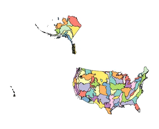
Here’s what the ecoregion map looks like so far, with Alaska and Hawaii in their true locations.
Image
Transforming Alaska
Now, let’s get only the rows from the TNC object that are part of Alaska, filtering by state %in% 'Alaska'. We use st_geometry() to pull out only the geometry column from the subsetted spatial data frame, then calculate the centroid of Alaska. To get the centroid we use st_union() to combine all the ecoregions into one shape, then st_centroid() to find its center point.
alaska <- tnc_map_trans %>% filter(state %in% 'Alaska')
alaska_g <- st_geometry(alaska)
alaska_centroid <- st_centroid(st_union(alaska_g))
Now for the actual transformations. We need to transform Alaska as follows:
- Rotate it by 39 degrees counterclockwise.
- Shrink it by a factor of 2.3.
- Move it to the east and south.
To rotate a geometric shape, we have to subtract its centroid so that the shape is centered around (0,0), multiply it by a rotation matrix, and then add the centroid back again. The function rot() I define here creates the transformation matrix for a given angle in radians.
rot <- function(a) matrix(c(cos(a), sin(a), -sin(a), cos(a)), 2, 2)
The sf package makes it really easy to apply all three transformations at once. We subtract the centroid, multiply by the rotation matrix for the angle -39 degrees (converted to radians), divide by 2.3, add back the centroid, then add a two-element vector to move all the points by a desired amount. If you don’t like the exact results you get from this, you can modify the parameters by changing the -39 to change the rotation, the 2.3 for the scaling, and the c(1000000, -5000000) for the relocation.
alaska_trans <- (alaska_g - alaska_centroid) * rot(-39 * pi/180) / 2.3 + alaska_centroid + c(1000000, -5000000)
Now we manually replace the geometry column in the alaska subsetted spatial data frame with the transformed geometry, and manually reassign the coordinate reference system (which was lost when we started messing with transformations).
alaska <- alaska %>% st_set_geometry(alaska_trans) %>% st_set_crs(st_crs(tnc_map_trans))
Transforming Hawaii
We do more or less the same thing for Hawaii, except that we rotate by 35 degrees counterclockwise, we don’t resize it at all, and we move it by a different amount. Again you can feel free to modify these parameters if you don’t like the result. (To resize it, multiply or divide before adding the centroid back again).
hawaii <- tnc_map_trans %>% filter(state %in% 'Hawaii')

hawaii_g <- st_geometry(hawaii)
hawaii_centroid <- st_centroid(st_union(hawaii_g))

hawaii_trans <- (hawaii_g - hawaii_centroid) * rot(-35 * pi/180) + hawaii_centroid + c(5200000, -1400000)
hawaii <- hawaii %>% st_set_geometry(hawaii_trans) %>% st_set_crs(st_crs(tnc_map_trans))
Putting it all together
Now all the pieces are in place. We create the final object by removing the original untransformed Alaska and Hawaii rows from the TNC map object, then bind the transformed Alaska and Hawaii objects to it.
tnc_map_final <- tnc_map_trans %>%
filter(!state %in% c('Alaska', 'Hawaii')) %>%
rbind(alaska) %>%
rbind(hawaii)
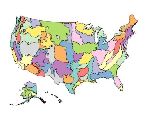
Check out our cool map!
Image
Code
To make it easier to copy-paste, all the code for the blog post is in one place in this R script.
Sources
Tutorial showing how to transform AK and HI with the sp package
Blog post showing how to make an interactive Covid map with transformed AK and HI
Share
Related Content
Making Free Maps with R, ggspatial, and Mapbox
Creating Visualizations with DiagrammeR
The interactive visualization gap in initial exploratory data analysis
Article published in IEEE Transactions on Visualization and Computer Graphics