Date
Description
Image
Overview
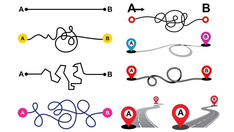
The fundamental definition of a “model” is an abstract representation of some object, idea, or process that can be physical, conceptual, or mathematical. People develop models for many different reasons—to understand a problem, to predict an outcome, to optimize a decision, to envision futures, or to bring people together to develop a shared understanding of an issue or system. Models present many pathways for attaining a desired outcome as illustrated in the cartoon at the top of this page. Models include only the essential features that are needed or that are useful for arriving at that outcome. The model’s level of complexity and the amount of information it needs depends on the particular reason for developing it.
Image
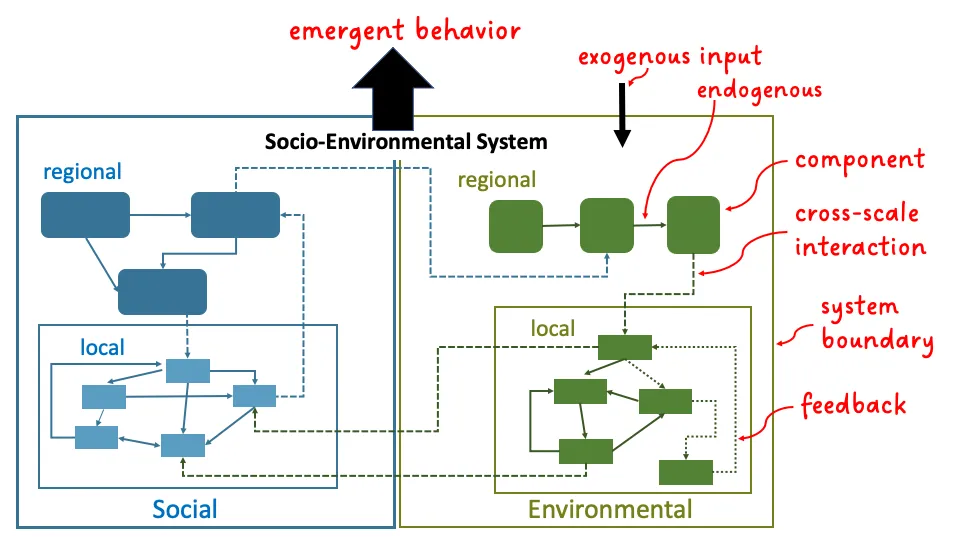
Socio-environmental systems (SES) focus on the dynamics between humans and the environment. They include multiple linked or interacting components/parts that together determine the overall behavior or state of those parts (Figure 2). Because many interactions and feedbacks are interdependent, we cannot easily predict the dynamics of the overall system, and thus we often say system behavior “emerges.”
Like economic markets and social networks, SES belong to a class of complex adaptive systems (CAS) that change and evolve over time. Modeling SES can be more difficult than modeling many other types of CAS because socio-environmental modeling requires bridging disciplines, scales, and data types to adequately represent the various social and biophysical processes. But like other CAS, SES are difficult to model because of the need to account for regime shifts that can fundamentally change a system’s dominant state and the way it operates. (See the Grand Challenges of SES Models video and Elsawah et al. 2020). Despite these challenges, SES models still offer a wealth of potential for better understanding the inherently complex coupled human-natural systems.
This explainer focuses primarily on SES models that use a variety of approaches. We have included common terms used by modelers at the end. An associated explainer provides information on different modeling approaches (e.g., system dynamics, agent-based, network) that may be used depending on the specific problem, context, and modeling goals.
A Few Modeling Basics
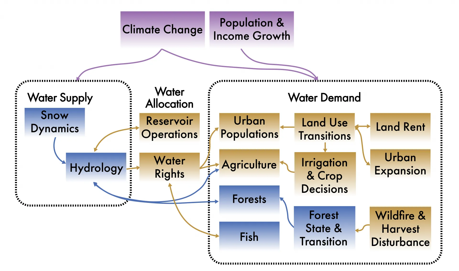
Computational models are powerful tools that have emerged with the advent of modern computing, and they are widely used in the sciences, including to understand SES (Schlüter et al. 2019). These models aim to simulate and study complex systems that would be impossible to understand through observation and experimentation alone. Researchers often use models in tandem with empirical observation, experimental design, hypothesis testing, and the development of fundamental theory. Models typically start with a conceptual diagram (Fig 3) that serves to define system boundaries; identify key parts of the system (components) at multiple scales; and predict system behavior that may emerge from interactions, feedbacks, and transformations. Identifying the relationships (called interactions, switches, or “flows”) between model components through visualized media is sometimes called ‘pseudocode.’ These simplified visual diagrams can help understand the complexity of the interactions and resulting feedbacks, especially for a SES. For example, the diagram below from Oregon State researchers (Jaeger et al. 2017) focuses on visualizing how climate change, population and economic growth may alter water availability and use in the Willamette River Basin (Figure 3).
Image
Once the relationships are mapped, the next step is defining those using mathematical equations, boolean (variables with true/false or 0/1 values) logic functions, or more qualitative strength relationships. For example, rural water demand (lnQRR) for the Willamette model pictured above is modeled as:
ln(QRR)= -3.55 – (0.6 ln(PC>)) + ln(Pop) + (0.13 ln(I)) - (0.048 ln(D))
PC is the “price” for water, Pop is the population of the rural residential unit, I is the average income per household, and D is people per sq. mi. Finally, some input data is inserted into these relationships in a given order and the output (e.g., QRR) can be interpreted.
Common Terms
- State variable: Used in dynamical (time-variant) models with iterative time steps. A variable (model component or part) whose “state” (i.e., value or other type of descriptor) can change over time (model iterations) as described by a set of “rules” or a functional equation describing the processes that contribute to the rate of change (e.g., dx/dt = f ….).
- Parameter: Any adjustable variable that is internal to a model’s operation and whose value can be estimated with empirical data or understanding of the system. Model parameters may be one or more constants such as coefficients in equations (e.g., a range in growth rates of forest cover).
- Calibration: The process of refining model parameter values to match observed or real-world data.
- Validation: Analysis of model accuracy in which model output is compared to real-world data produced under conditions similar to those in the simulation or by comparing model output to a reserved subset of data not used to calibrate or parameterize the original model.
- Feedback: Aspect of dynamical models in which the value or behavior of one variable (variable A) influences the value or behavior of one of variable A’s input variables (variable B).
- Differential equation: Equations that deal with the relationship of a physical quantity and its continuous change over time. Used in creating dynamic simulation models. Note, difference equations are sometimes used which rely on discrete time steps.
- Boolean function: A function whose argument consists of a logical, binary output, often true or false—a variable may be either “on” or “off”, relevant or not, 0 or 1.
- Probabilistic: Based on the probability of something occurring, often including a range of possible outcomes whose likelihood of occurrence is decided by assigning it a probability value.
- Global vs. local: Global models simulate output by using all ranges or samples of data and observations while a local model only considers a subset of that data, sometimes used for validation purposes.
- Sensitivity analysis: An investigation into how the uncertainty of a model output can be attributed to differences in the uncertainty among a model’s input parameters.
- Metamodel: An abstract, simplified version of a full model often used to reduce computational demands of a model to facilitate model execution or to be combined with another model.
- System boundary: Limits or constraints of input variables imposed on a model often related to spatial and temporal scales. Boundaries are often drawn in early development and diagramming of a model based on a modeling team’s interests and goals. Boundaries can define what items are endogenous (those explicitly simulated in a model) or exogenous (those whose input is used in model simulation, but whose values are predetermined, not simulated e.g., temperature or rainfall in an ecosystem model). Boundaries can also define what variables are considered or omitted (variables deemed trivial or not well enough understood to model accurately and therefore left out).
- Static vs. dynamic model: A static model represents a system at a particular point in time while dynamic models simulate changes over time using differential or difference equations.
- Steady state: Model state in which inputs and outputs are balanced resulting in unchanging (i.e., steady) state variables.
- Regime shift: Large-scale state changes in socio-environmental systems often caused by chronic or stochastic pressures or disturbance, that leads to fundamentally different structure and function of the given system.
References
- Elsawah, S., Filatova, T., Jakeman, A.J. et al. (2020). Eight grand challenges in socio-environmental systems modeling. Socio-Environmental Systems Modelling, 2. https://doi.org/10.18174/sesmo.2020a16226
- Jaeger, W.K., Amos, A., Bigelow, D.P. et al. (2017). Finding water scarcity amid abundance using human–natural system models. Proceedings of the National Academy of Sciences, 114(45), 11884-11889. https://doi.org/10.1073/pnas.1706847114
- Schlüter, M., Haider, L.J., Lade, S.J. et al. (2019). Capturing emergent phenomena in social-ecological systems: an analytical framework. Ecology and Society, 24(3), 11. https://doi.org/10.5751/ES-11012-240311
Share